# Uncomment to run the notebook in Colab
# ! pip install -q "wax-ml[complete]@git+https://github.com/eserie/wax-ml.git"
# ! pip install -q --upgrade jax jaxlib==0.1.70+cuda111 -f https://storage.googleapis.com/jax-releases/jax_releases.html

# check available devices
import jax

print("jax backend {}".format(jax.lib.xla_bridge.get_backend().platform))
jax.devices()

WARNING:absl:No GPU/TPU found, falling back to CPU. (Set TF_CPP_MIN_LOG_LEVEL=0 and rerun for more info.)
WARNING:absl:No GPU/TPU found, falling back to CPU. (Set TF_CPP_MIN_LOG_LEVEL=0 and rerun for more info.)

jax backend cpu

[CpuDevice(id=0)]

〰 Compute exponential moving averages with xarray and pandas accessors 〰

WAX-ML implements pandas and xarray accessors to ease the usage of machine-learning algorithms with high-level data APIs :

• pandas’s DataFrame and Series

• xarray’s Dataset and DataArray.

These accessors allow to easily execute any function using Haiku modules on these data containers.

For instance, WAX-ML propose an implementation of the exponential moving average realized with this mechanism.

Let’s show how it works.

Load accessors

First you need to load accessors:

from wax.accessors import register_wax_accessors

register_wax_accessors()

EWMA on dataframes

Let’s look at a simple example: The exponential moving average (EWMA).

Let’s apply the EWMA algorithm to the NCEP/NCAR ‘s Air temperature data.

🌡 Load temperature dataset 🌡

import xarray as xr

dataset = xr.tutorial.open_dataset("air_temperature")

Let’s see what this dataset looks like:

dataset

<xarray.Dataset>
Dimensions:  (lat: 25, lon: 53, time: 2920)
Coordinates:
  * lat      (lat) float32 75.0 72.5 70.0 67.5 65.0 ... 25.0 22.5 20.0 17.5 15.0
  * lon      (lon) float32 200.0 202.5 205.0 207.5 ... 322.5 325.0 327.5 330.0
  * time     (time) datetime64[ns] 2013-01-01 ... 2014-12-31T18:00:00
Data variables:
    air      (time, lat, lon) float32 ...
Attributes:
    Conventions:  COARDS
    title:        4x daily NMC reanalysis (1948)
    description:  Data is from NMC initialized reanalysis\n(4x/day).  These a...
    platform:     Model
    references:   http://www.esrl.noaa.gov/psd/data/gridded/data.ncep.reanaly...

To compute a EWMA on some variables of a dataset, we usually need to convert data in pandas series or dataframe.

So, let’s convert the dataset into a dataframe to illustrate accessors on a dataframe:

dataframe = dataset.air.to_series().unstack(["lon", "lat"])

EWMA with pandas

air_temp_ewma = dataframe.ewm(alpha=1.0 / 10.0).mean()
_ = air_temp_ewma.iloc[:, 0].plot()

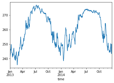
EWMA with WAX-ML

air_temp_ewma = dataframe.wax.ewm(alpha=1.0 / 10.0).mean()
_ = air_temp_ewma.iloc[:, 0].plot()

On small data, WAX-ML’s EWMA is slower than Pandas’ because of the expensive data conversion steps. WAX-ML’s accessors are interesting to use on large data loads (See our three-steps_workflow)

Apply a custom function to a Dataset

Now let’s illustrate how WAX-ML accessors work on xarray datasets.

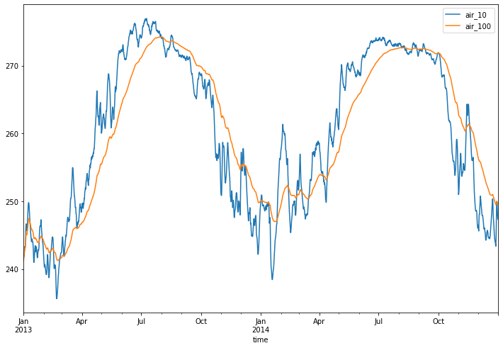
from wax.modules import EWMA


def my_custom_function(dataset):
    return {
        "air_10": EWMA(1.0 / 10.0)(dataset["air"]),
        "air_100": EWMA(1.0 / 100.0)(dataset["air"]),
    }


dataset = xr.tutorial.open_dataset("air_temperature")
output, state = dataset.wax.stream().apply(
    my_custom_function, format_dims=dataset.air.dims
)

_ = output.isel(lat=0, lon=0).drop(["lat", "lon"]).to_pandas().plot(figsize=(12, 8))